DaSPi

daspi

Data analysis, Statistics and Process improvements (DaSPi)

Visualize and analyze your data with DaSPi. This package is designed for users who want to find relevant influencing factors in processes and validate improvements. This package offers many Six Sigma tools based on the following packages:

• pandas
• numpy
• matplotlib
• scipy
• statsmodels

The goal of this package is to be easy to use and flexible so that it can be adapted to a wide array of data analysis tasks.

Why DaSPi?

There are great packages for data analysis and visualization in Python, such as Pandas, Seaborn, Altair, Statsmodels, Scipy, Pinguins. But most of the time they work not directly with each other. Wouldn't it be great if you could use all of these packages together in one place? That's where DaSPi comes in. DaSPi is a Python package that provides a unified interface for data analysis, statistics and visualization. It allows you to use all of the great packages mentioned above together in one place, making it easier to explore and understand your data.

Features

• Ease of Use: DaSPi is designed to be easy to use, even for beginners. It provides a simple and intuitive interface that makes it easy to get started with data analysis.
• Visualization: DaSPi provides a wide range of visualization options, including multivariate charts, joint charts, and useful precast. This makes it easy to explore and understand your data in a visual way.
• Statistics: DaSPi provides a wide range of statistical functions and tests, including hypothesis testing, confidence intervals, and regression analysis. This makes it easy to explore and understand your data in a statistical way.
• Open Source: DaSPi is open source, which means that it is free to use and modify. This makes it a great option for users who want to customize the package to their specific needs.

This Package contains following submodules:

• plotlib: Visualizations with Matplotlib, where the division by color, marker size or shape as well as rows and columns subplots are automated depending on the given categorical data. Any plots can also be combined, such as scatter with contour plot, violin with error bars or other creative combinations.
• anova: analysis of variance (ANOVA), which is used to compare the variance within and between of two or more groups, or the effects of different treatments on a response variable. It also includes a function for calculating the variance inflation factor (VIF) for linear regression models. The main class is LinearModel, which provides methods for fitting linear regression with interactions and automatically elimiinating insignificant variables.
• statistics: applied statistics, hypothesis test, confidence calculations and monte-carlo simulation. It also includes estimation for process capability and capability index.
• datasets: data for exersices. It includes different datasets that can be used for testing and experimentation.

Usage

Visualization

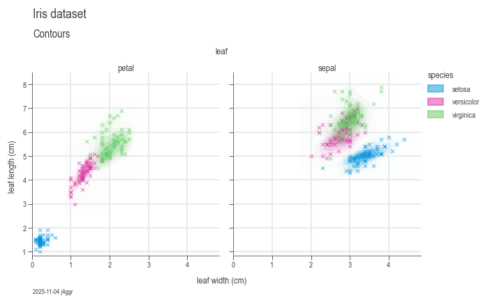
To use DaSPi, you can import the package and start exploring your data. Here is an example of how to use DaSPi to visualize a dataset:

import daspi as dsp
df = dsp.load_dataset('iris')

chart = dsp.MultivariateChart(
        source=df,
        target='length',
        feature='width',
        hue='species',
        col='leaf',
        markers=('x',)
    ).plot(
        dsp.GaussianKDEContour
    ).plot(
        dsp.Scatter
    ).label(
        feature_label='leaf width (cm)',
        target_label='leaf length (cm)',
    )

ANOVA

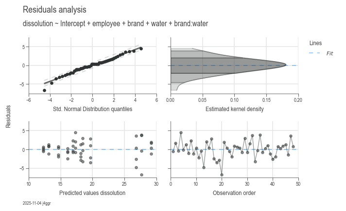
Do some ANOVA and statistics on a dataset. Run the example below in a Jupyther Notebook to see the results.

df = dsp.load_dataset('painkillers-dissolution')
model = dsp.LinearModel(
    source=df,
    target='dissolution',
    features=['employee', 'stirrer', 'brand', 'catalyst', 'water'],
    covariates=['temperature', 'preparation'],
    order=2)
df_gof = pd.concat(model.recursive_elimination())

dsp.ResidualsCharts(model).plot().stripes().label(info=True)
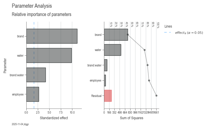
dsp.ParameterRelevanceCharts(model).plot().label(info=True)
model

Formula:

dissolution ~ 16.0792 + 2.3750 employee[T.B] + 0.8375 employee[T.C] + 10.7500 brand[T.OuchAway] - 3.8000 water[T.tap] - 5.7167 brand[T.OuchAway]:water[T.tap]

Model Summary

Hierarchical	Least Parameter	P Least	S	AIC	R²	R² Adj	R² Pred
True	employee	0.023298	2.374693	224.835935	0.857379	0.840400	0.813719

Parameter Statistics

	Coef	Std Err	T	P	CI Low	CI Upp
Intercept	16.079167	0.839581	19.151424	0.000000	14.384824	17.773509
employee[T.B]	2.375000	0.839581	2.828793	0.007133	0.680657	4.069343
employee[T.C]	0.837500	0.839581	0.997522	0.324224	-0.856843	2.531843
brand[T.OuchAway]	10.750000	0.969464	11.088598	0.000000	8.793542	12.706458
water[T.tap]	-3.800000	0.969464	-3.919690	0.000321	-5.756458	-1.843542
brand[T.OuchAway]:water[T.tap]	-5.716667	1.371030	-4.169616	0.000149	-8.483516	-2.949817

Analysis of Variance

Source	DF	SS	MS	F	P	n²
employee	2	46.431667	23.215833	4.116891	0.023298	0.027960
brand	1	747.340833	747.340833	132.526821	0.000000	0.450027
water	1	532.000833	532.000833	94.340328	0.000000	0.320355
brand:water	1	98.040833	98.040833	17.385695	0.000149	0.059037
Residual	42	236.845000	5.639167	nan	nan	0.142621

Variance Inflation Factor

	DF	VIF	GVIF	Threshold	Collinear	Method
Intercept	1	5.000000	2.236068	2.236068	True	R_squared
employee	2	1.000000	1.000000	1.495349	False	generalized
brand	1	1.000000	1.000000	2.236068	False	R_squared
water	1	1.000000	1.000000	2.236068	False	R_squared
brand:water	1	1.000000	1.000000	2.236068	False	single_order-2_term

Process capability

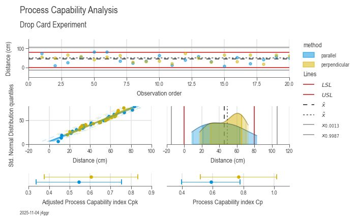
Analyze process variation and other key performance indicators for process capacity.

df = dsp.load_dataset('drop_card')
spec_limits = dsp.SpecLimits(0, float(df.loc[0, 'usl']))
target = 'distance'

chart = dsp.ProcessCapabilityAnalysisCharts(
        source=df,
        target=target,
        spec_limits=spec_limits,
        hue='method'
    ).plot(
    ).stripes(
    ).label(
        fig_title='Process Capability Analysis',
        sub_title='Drop Card Experiment',
        target_label='Distance (cm)',
        info=True
    )

samples_parallel = df[df['method']=='parallel'][target]
samples_series = df[df['method']=='perpendicular'][target]
pd.concat([
    dsp.ProcessEstimator(samples_parallel, spec_limits).describe(),
    dsp.ProcessEstimator(samples_series, spec_limits).describe()],
    axis=1,
    ignore_index=True,
).rename(
    columns={0: 'parallel', 1: 'perpendicular'}
)

	parallel	perpendicular
n_samples	20	20
n_missing	0	0
n_ok	18	20
n_nok	2	0
n_errors	0	0
ok	90.00 %	100.00 %
nok	10.00 %	0.00 %
nok_norm	8.01 %	3.73 %
nok_fit	7.24 %	5.77 %
min	8.5	17.5
max	83.0	73.0
mean	42.935	48.485
median	40.75	52.5
std	22.666583	17.359489
sem	5.068402	3.8817
excess	-0.900801	-1.236078
p_excess	0.288757	0.072573
skew	0.19252	-0.377538
p_skew	0.690373	0.438723
p_ad	0.754044	0.098371
dist	lognorm	logistic
p_ks	0.964797	0.744326
strategy	norm	norm
lcl	-25.064748	-3.593468
ucl	110.934748	100.563468
lsl	0	0
usl	80.0	80.0
cp	0.588237	0.768072
cpk	0.545076	0.605145
Z	1.635227	1.815434
Z_lt	0.135227	0.315434

About DaSPi

DaSPi was created and is actively maintained by Reto Jäggli, a Data Scientist at Festo Microtechnology AG. Much of the development happens during spare time, driven by a passion for making data analysis, statistics, and process improvement more accessible and integrated.

Contributions to DaSPi are very welcome! If you find bugs or have ideas for improvements, please report them or submit pull requests on the GitHub repository, where the full source code is also available for review.

Important Notice:
DaSPi is still under heavy development and may contain hidden bugs. While every effort is made to ensure reliability, no warranty is provided. The results obtained using DaSPi should be double-checked with other trusted statistical software whenever possible. Where applicable, DaSPi acts as a convenient wrapper around well-established packages such as pandas, numpy, matplotlib, scipy, and statsmodels, leveraging their robustness and functionality.