Gage R&R Guide¶

Introduction¶

Measurement System Analysis (MSA) is a critical component of quality management and process improvement. It provides methods to evaluate and quantify the variation in a measurement system, ensuring that your measurement process is capable and reliable before making decisions based on the data it produces.

This guide covers the complete workflow for gage analysis in DaSPi, including:

Gage Study (MSA Type 1): Evaluates the measurement system itself using a single reference
Gage R&R (MSA Type 2 & 3): Evaluates repeatability and reproducibility with multiple parts and operators

Why Measurement System Analysis Matters¶

Before analyzing process variation, you must ensure your measurement system is capable. A poor measurement system can lead to:

Incorrect conclusions about process capability
Wrong decisions about product conformance
Wasted resources investigating "problems" that don't exist
Failure to detect real quality issues

The golden rule: Measurement variation should be small compared to process variation and specification limits.

Standard Uncertainty Components¶

The following table shows the typical standard uncertainties as they affect measurements. They are divided into Measurement System (MS) and Measurement Process (MP). The individual standard uncertainty components can be determined using method A or B. The method B refers to prior knowledge or information from manuals or specifications and the method A refers to statistical analysis.

Shortcut	Uncertainty Component	Impact	Method
`CAL`	Calibration of the reference	MS	B
`RE`	Display resolution	MS	B
`BI`	Bias	MS	A/B
`LIN`	Linearity deviation	MS	A/B
`EVR`	Equipment Variation (repeatability) on the reference	MS	A
`MPE`	Maximum Permissible Error (error limit)	MS	B
`EVO`	Equipment Variation (repeatability) on the object	MP	A
`AV`	Appraiser Variation (comparability of operators)	MP	A
`GV`	Gage Variation (comparability of measurement system)	MP	A
`IA`	Interactions	MP	A
`T`	Temperature	MP	A/B
`STAB`	Stability over time	MP	A
`OBJ`	Inhomogeneity of the object	MP	A/B
`REST`	Other uncertainties not covered by the above	MS/MP	B

MSA Type 1: Gage Study¶

Overview¶

A Gage Study (MSA Type 1) evaluates the measurement system using repeated measurements of one or more reference standards. This is the foundation for understanding your measurement system's basic performance.

When to Use¶

Qualifying a new measurement system
Verifying measurement system performance over time
Determining measurement uncertainty for a single gage
Checking for bias and linearity across the measurement range

Quick Start Example¶

import daspi as dsp

# Load example data
df = dsp.load_dataset('grnr_adjustment')

# Create a GageEstimator for a single reference
gage = dsp.GageEstimator(
    samples=df['result_gage'],
    reference=df['reference'][0],      # True reference value
    u_cal=df['U_cal'][0],              # Calibration uncertainty
    tolerance=df['tolerance'][0],       # Specification tolerance
    resolution=df['resolution'][0]      # Gage resolution
)

# View the results
print(gage.describe())

Understanding the Output¶

The GageEstimator provides several key metrics:

import daspi as dsp
df = dsp.load_dataset('grnr_adjustment')
gage = dsp.GageEstimator(
    samples=df['result_gage'],
    reference=df['reference'][0],
    u_cal=df['U_cal'][0],
    tolerance=df['tolerance'][0],
    resolution=df['resolution'][0]
)
print(gage.describe())

	result_gage
n_samples	60.00000
n_missing	6.00000
n_outlier	0.00000
min	1.00070
max	1.00160
R	0.00090
mean	1.00081
median	1.00080
std	0.00013
sem	0.00002
p_ad	9.866e-20
lower	0.98700
upper	1.01300
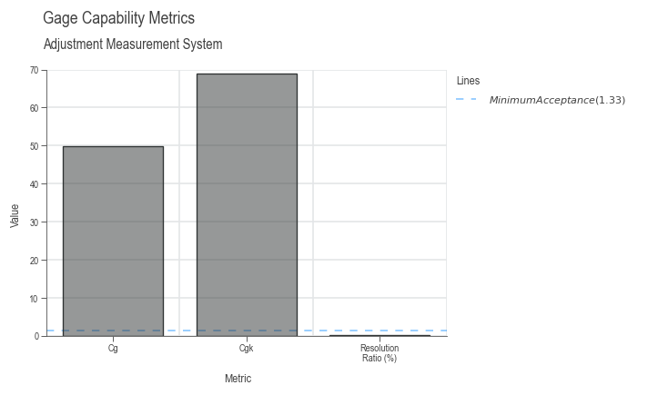
cg	49.73226
cgk	68.99967
bias	0.00081
p_bias	3.723e-44
T_min_cg	0.00235
T_min_cgk	0.01044
T_min_res	0.00200
resolution_ratio	0.00077

Metrics explained:

n_samples: Number of measurements taken
mean: Average of all measurements
std: Standard deviation (repeatability)
bias: Difference between mean and reference (mean - reference)
p_bias: Statistical significance of bias (p-value)
Cg: Capability index for variation (similar to Cp)
Cgk: Capability index considering bias (similar to Cpk)
resolution_ratio: Resolution as proportion of tolerance

Acceptance Criteria (typical values):

Cg, Cgk ≥ 1.33: Measurement system is acceptable
1.00 ≤ Cg, Cgk < 1.33: Marginal, may be acceptable depending on application
Cg, Cgk < 1.00: Unacceptable, measurement system needs improvement
resolution_ratio < 0.05: Resolution is adequate (5% rule)

Gage Capability Metrics

Multiple Reference Standards (Linearity Check)¶

To evaluate linearity across the measurement range, use multiple reference standards:

import daspi as dsp

# Load data with multiple reference parts
df = dsp.load_dataset('grnr_layer_thickness')

# Create GageStudyModel with linearity evaluation
gage = dsp.GageStudyModel(
    source=df,
    target='result_gage',
    reference='reference',
    u_cal=df['U_cal'][0],
    tolerance=df['tolerance'][0],
    resolution=df['resolution'][0],
    bias_corrected=False  # Include bias in uncertainty
)

# Create visualization
chart = dsp.GageStudyCharts(
    gage, 
    stretch_figsize=1.5
).plot().stripes().label()

# Display model summary
gage

What gets calculated:

Individual bias for each reference level
Linearity uncertainty (u_lin)
Combined measurement system uncertainty
Capability indices for each reference

The output tables include:

References Analysis:

	Ref	mean	Bias	s	R
1	0.101000	0.100660	-0.000340	0.000688	0.003000

Gage capability:

	Value	Limit	Capable	T_min
Cg	2.179005	1.330000	True	0.018311
Cgk	1.932051	1.330000	True	0.021711
RE_ratio	0.033333	0.050000	True	0.020000
Q_MS	0.096371	0.150000	True	0.019274
p_BI	0.001024	0.050000	False	nan

Measurement uncertainty budget measuring process:

	u	U	Q	rank
CAL	0.000100	0.000200	0.013333	4.000000
RE	0.000289	0.000577	0.038490	2.000000
BI	0.000196	0.000393	0.026173	3.000000
LIN	0.000000	0.000000	0.000000	nan
EVR	0.000688	0.001377	0.091785	1.000000
REST	0.000000	0.000000	0.000000	nan
MS	0.000723	0.001446	0.096371	nan

Gage Study Single Reference

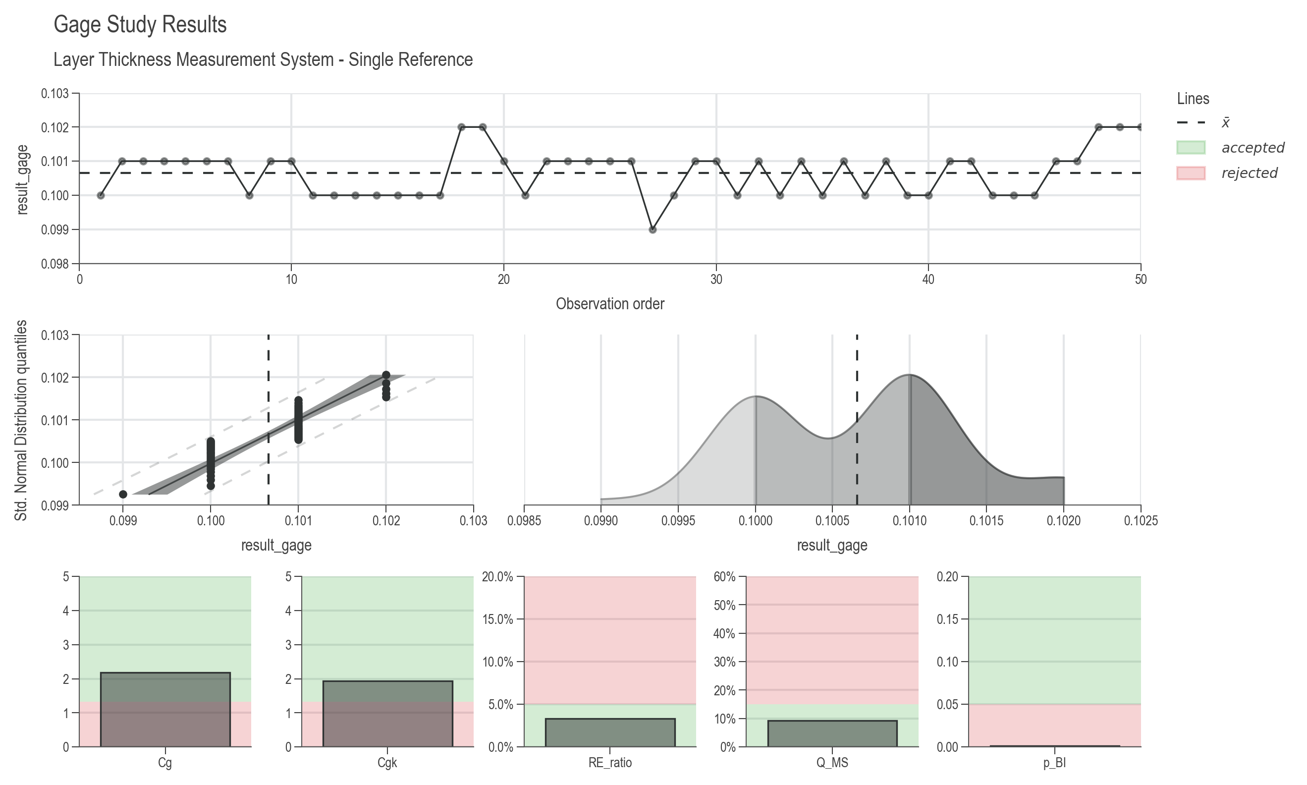
Visualizing Gage Study Results¶

The GageStudyCharts class creates a comprehensive dashboard with:

Measurements by Reference: Shows variation at each reference level
Probability Plot: Checks normality of measurement errors
Distribution: Shows the shape of the measurement distribution
Capability Indices: Bar charts showing Cg, Cgk, resolution ratio, etc.

# Customize the chart appearance
chart = dsp.GageStudyCharts(gage, stretch_figsize=1.5)
chart.plot()      # Create all plots
chart.stripes()   # Add reference lines and zones
chart.label(      # Add labels and titles
    fig_title='Gage Study Results',
    sub_title='Layer Thickness Measurement System'
)
# chart.save('gage_study_results.png')  # Optionally save

Working with Measurement Uncertainty¶

The GageStudyModel calculates a complete uncertainty budget:

# Access individual uncertainty components
print(f"Calibration uncertainty (u_cal): {gage.u_cal.expanded:.6f}")
print(f"Resolution uncertainty (u_re): {gage.u_re.expanded:.6f}")
print(f"Bias uncertainty (u_bi): {gage.u_bi.expanded:.6f}")
print(f"Linearity uncertainty (u_lin): {gage.u_lin.expanded:.6f}")
print(f"Repeatability uncertainty (u_evr): {gage.u_evr.expanded:.6f}")

# Combined measurement system uncertainty
print(f"\nCombined MS uncertainty: {gage.u_ms.expanded:.6f}")

# Check if measurement system is capable
print(f"Q_MS ratio: {gage.u_ms.expanded / gage.tolerance * 2:.4f}")
print(f"Acceptable if Q_MS < {gage.q_ms_limit}")

The Q_MS ratio indicates the proportion of tolerance consumed by measurement uncertainty. A typical limit is 0.15 (15%), meaning measurement uncertainty should not exceed 15% of the tolerance.

Coverage Factor (k)¶

The coverage factor determines the confidence level of the uncertainty:

k = 2: ~95% confidence interval (default)
k = 3: ~99.7% confidence interval

# Change coverage factor
gage.k = 3
print(f"Expanded uncertainty (k=3): {gage.u_ms.expanded:.6f}")

MSA Type 2 & 3: Gage R&R Study¶

Overview¶

Gage R&R (Repeatability and Reproducibility) extends the gage study to evaluate variation across multiple parts, operators, and/or measurement systems. This provides a comprehensive view of measurement process variation.

Repeatability (EV): Variation when the same operator measures the same part multiple times
Reproducibility (AV or GV): Variation between different operators or measurement systems
Interactions: Part-operator interactions that affect measurements

When to Use¶

MSA Type 2: Multiple operators measure multiple parts (evaluates operator variation)
MSA Type 3: Multiple measurement conditions without operator influence (e.g., different fixtures, locations, temperatures)

Complete Gage R&R Example¶

import daspi as dsp

# Load dataset
df = dsp.load_dataset('grnr_layer_thickness')

# Step 1: Create the Gage Study (MSA Type 1)
gage = dsp.GageStudyModel(
    source=df,
    target='result_gage',
    reference='reference',
    u_cal=df['U_cal'][0],
    tolerance=df['tolerance'][0],
    resolution=df['resolution'][0]
)

# Step 2: Create the Gage R&R Model
model = dsp.GageRnRModel(
    source=df,
    target='result_rnr',
    part='part',           # Column identifying different parts
    gage=gage,             # GageStudyModel from Step 1
    u_av='operator'        # Column identifying operators (Type 2)
    # u_gv='fixture'       # Use this instead for Type 3
)

# Step 3: Visualize Results
chart = dsp.GageRnRCharts(
    model, 
    stretch_figsize=True
).plot().stripes().label()

# Step 4: Review the model
model  # Displays comprehensive uncertainty budget

Understanding Gage R&R Output¶

The GageRnRModel provides several tables:

1. ANOVA Table¶

Shows the statistical analysis of variance sources:

print(model.anova())

Example output:

Typ-I	DF	SS	MS	F	p	n2
Source
part	9	0.001588	0.000176	261.907904	0.000000	0.979539
operator	2	0.000001	0.000000	0.618557	0.542960	0.000514
Residual	48	0.000032	0.000001	nan	nan	0.019947

Key sources of variation:

Part: Variation between different parts (desired variation)
Operator: Variation due to operators/systems
Part×Operator: Interaction effects
Residual: Repeatability (pure measurement variation)

Columns explained:

DF: Degrees of freedom
SS: Sum of squares
MS: Mean squares
F: F-statistic
p: p-value for significance
n2: Proportion of total variance explained

2. Gage R&R Table¶

print(model.rnr())

Shows the variance components breakdown:

Repeatability and reproducibility (R&R):

	MS	MS/Total	s	6s	6s/Total	6s/Tolerance
R&R	0.000001	0.022480	0.000821	0.004924	0.149932	0.164148
EV	0.000001	0.022480	0.000821	0.004924	0.149932	0.164148
AV	0.000000	0.000000	0.000000	0.000000	0.000000	0.000000
PV	0.000029	0.977520	0.005412	0.032473	0.988696	1.082437
Total	0.000030	1.000000	0.005474	0.032844	1.000000	1.094812

Interpretation:

R&R < 10%: Excellent
10% ≤ R&R < 30%: Acceptable
R&R ≥ 30%: Unacceptable
PV should dominate the variation
EV should be small compared to PV
AV should be minimal or zero if operators are consistent

Columns explained:

MS: Mean square from ANOVA
MS/Total: Proportion of total variance
s: Standard deviation for each source
6s: Six times the standard deviation (approximate range)
6s/Total: Proportion of total variation
6s/Tolerance: Proportion of tolerance consumed by each source

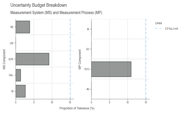
3. Uncertainty Budget¶

print(model.uncertainties())

Provides a complete breakdown of all uncertainty components:

Measurement uncertainty budget:

	u	U	Q	rank
CAL	0.000100	0.000200	0.013333	5.0
RE	0.000289	0.000577	0.038490	3.0
BI	0.000196	0.000393	0.026173	4.0
LIN	0.000000	0.000000	0.000000	NaN
EVR	0.000688	0.001377	0.091785	2.0
MS_REST	0.000000	0.000000	0.000000	NaN
MS	0.000723	0.001446	0.096371	NaN
EVO	0.000821	0.001641	0.109432	1.0
AV	0.000000	0.000000	0.000000	NaN
GV	0.000000	0.000000	0.000000	NaN
IA	0.000000	0.000000	0.000000	NaN
T	0.000000	0.000000	0.000000	NaN
STAB	0.000000	0.000000	0.000000	NaN
OBJ	0.000000	0.000000	0.000000	NaN
MP_REST	0.000000	0.000000	0.000000	NaN
MP	0.000850	0.001700	0.113305	NaN

Measurement System (MS): CAL, RE, BI, LIN, EVR, REST
Measurement Process (MP): EVO, AV, GV, IA, T, STAB, OBJ, REST

Each component shows:

Standard uncertainty (u)
Expanded uncertainty (U) at coverage factor k
Proportion (Q) relative to tolerance
Rank: Importance of each component

Uncertainty Budget Breakdown

Customizing Gage R&R Analysis¶

Bias Correction¶

If you identify and correct for bias, set bias_corrected=True:

gage = dsp.GageStudyModel(
    source=df,
    target='result_gage',
    reference='reference',
    u_cal=df['U_cal'][0],
    tolerance=df['tolerance'][0],
    resolution=df['resolution'][0],
    bias_corrected=True  # Bias is corrected, don't include in uncertainty
)

Additional Uncertainty Sources¶

Include temperature, stability, or object inhomogeneity:

# Method A: From data (categorical column)
model = dsp.GageRnRModel(
    source=df,
    target='result_rnr',
    part='part',
    gage=gage,
    u_av='operator',
    u_t='temperature',      # Temperature effect from data
    u_stab='time_period',   # Stability over time from data
    u_obj='location'        # Object inhomogeneity from data
)

# Method B: From prior knowledge
from daspi.statistics.confidence import MeasurementUncertainty

u_temp = MeasurementUncertainty(
    error_limit=0.005,      # ±0.005 variation due to temperature
    distribution='rectangular',
    k=2
)

model = dsp.GageRnRModel(
    source=df,
    target='result_rnr',
    part='part',
    gage=gage,
    u_av='operator',
    u_t=u_temp              # Known temperature uncertainty
)

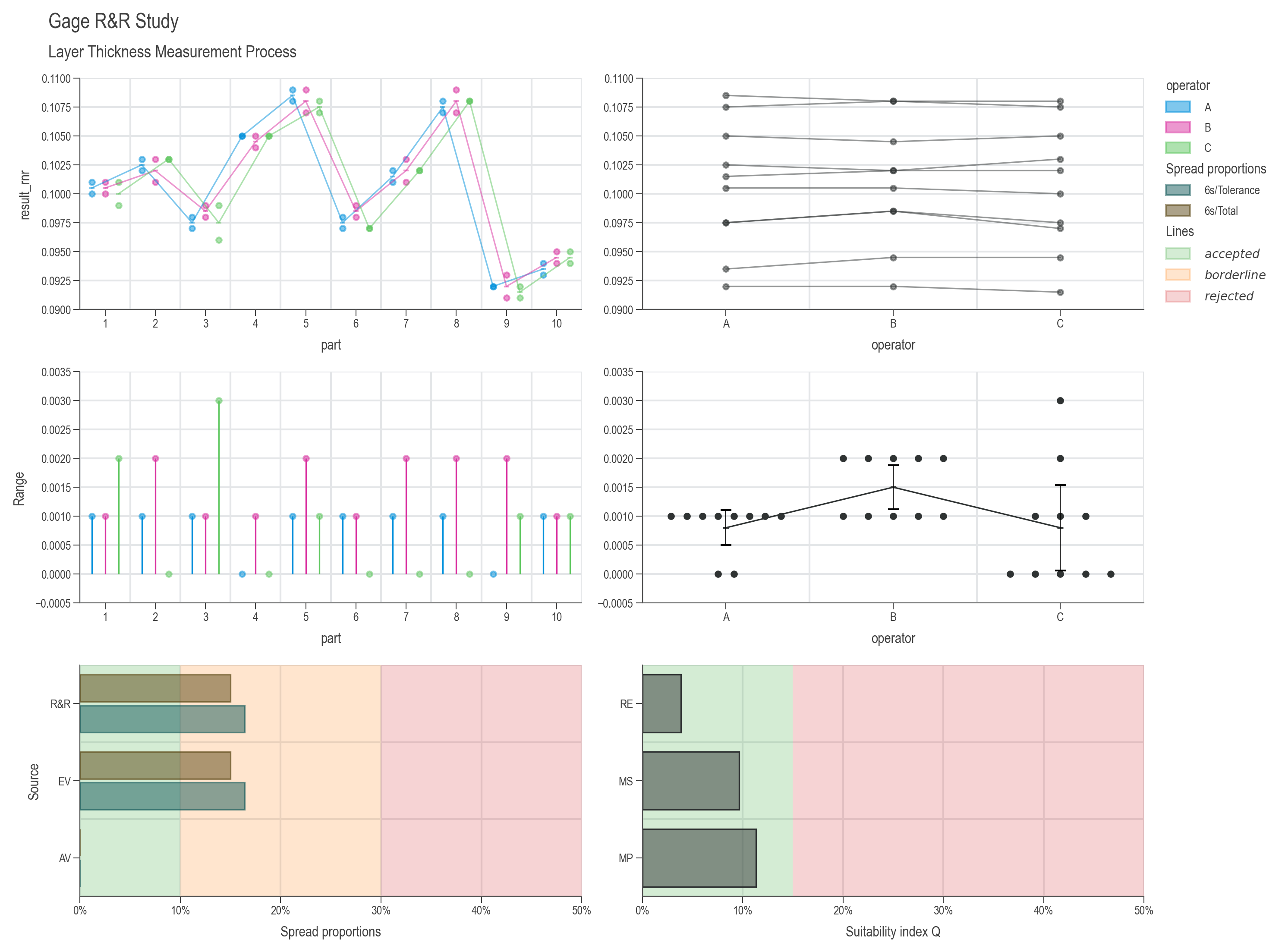
Visualizing Gage R&R Results¶

The GageRnRCharts creates six diagnostic plots:

Measurement by Part (by Operator): Shows part-to-part variation
Measurement by Operator: Shows operator consistency across parts
Range by Part: Shows within-part repeatability
Range by Operator: Shows operator repeatability
Variance Components (%Spread and %Tol): Bar chart comparing sources
Uncertainty Budget: Shows MS, MP, and total measurement uncertainty

chart = dsp.GageRnRCharts(
    model,
    spread_accepted_limit=0.1,   # 10% threshold for acceptance
    spread_rejected_limit=0.3,   # 30% threshold for rejection
    u_accepted_limit=0.15,       # 15% uncertainty threshold
    stretch_figsize=True
)

chart.plot()
chart.stripes()  # Adds acceptance zones
chart.label(
    fig_title='Gage R&R Study',
    sub_title='Layer Thickness Measurement Process'
)
# chart.save('docs/img/gage_rnr_layer_thickness.png')

Gage R&R Layer Thickness

Practical Workflow¶

Step-by-Step Process¶

MSA Decision Flow

1. Define Your Measurement System

Identify the gage/instrument
Determine specification limits
Know calibration uncertainty
Understand resolution

2. Collect Data

For Gage Study (Type 1):

Measure reference standard(s) multiple times (≥ 25-50 measurements)
Use multiple references across the measurement range for linearity

For Gage R&R (Type 2):

Select representative parts (≥ 10 parts spanning the range)
Have multiple operators (≥ 2-3 operators)
Each operator measures each part multiple times (≥ 2-3 trials)
Randomize measurement order

3. Analyze with DaSPi

# Type 1: Gage Study
gage = dsp.GageStudyModel(source, target, reference, ...)

# Type 2/3: Gage R&R
model = dsp.GageRnRModel(source, target, part, gage, u_av, ...)

4. Interpret Results

Check acceptance criteria:

Cg, Cgk ≥ 1.33
%Spread < 10% (excellent) or < 30% (acceptable)
Q_MS < 0.15 (measurement uncertainty < 15% of tolerance)

5. Take Action

If measurement system is unacceptable:

Improve resolution (better gage)
Reduce bias (calibration, correction)
Improve repeatability (better fixturing, procedure)
Reduce operator variation (training, standardization)
Control environmental factors (temperature, vibration)

Data Requirements¶

Gage Study Dataset Structure¶

# Columns needed for GageStudyModel:
# - target: measurement results (e.g., 'result_gage')
# - reference: reference value for each measurement
# - Additional: tolerance, resolution, calibration uncertainty (can be constants)

Example:

   result_gage  reference  tolerance  resolution  U_cal
0       0.1000      0.101       0.03       0.001  0.0002
1       0.1010      0.101        NaN         NaN     NaN
2       0.1010      0.101        NaN         NaN     NaN
...

Gage R&R Dataset Structure¶

# Columns needed for GageRnRModel:
# - target: measurement results (e.g., 'result_rnr')
# - part: part identifier
# - operator: operator identifier (Type 2) OR
# - other categorical columns for Type 3 (fixture, location, etc.)

Example:

   result_rnr  part  operator  trial
0       0.107     8         A      1
1       0.105     4         A      1
2       0.092     9         A      1
...

Common Use Cases¶

Use Case 1: New Measurement System Qualification¶

# Collect 50 measurements on a single reference
df = collect_gage_data(reference_value=10.0, n_measurements=50)

gage = dsp.GageEstimator(
    samples=df['measurement'],
    reference=10.0,
    u_cal=0.002,
    tolerance=0.1,
    resolution=0.001
)

# Check if acceptable
if gage.cg >= 1.33 and gage.cgk >= 1.33:
    print("Measurement system is qualified!")
else:
    print("Measurement system needs improvement")

Use Case 2: Periodic Verification¶

# Check gage performance quarterly
df = dsp.load_dataset('grnr_adjustment')

gage = dsp.GageEstimator(
    samples=df['result_gage'],
    reference=df['reference'][0],
    u_cal=df['U_cal'][0],
    tolerance=df['tolerance'][0],
    resolution=df['resolution'][0]
)

# Compare to historical baseline
if gage.std > historical_std * 1.2:
    print("WARNING: Repeatability has degraded")

Use Case 3: Operator Training Effectiveness¶

# Evaluate operators before and after training
model_before = dsp.GageRnRModel(df_before, 'measurement', 'part', gage, u_av='operator')
model_after = dsp.GageRnRModel(df_after, 'measurement', 'part', gage, u_av='operator')

av_before = model_before.u_av.expanded
av_after = model_after.u_av.expanded

improvement = (av_before - av_after) / av_before * 100
print(f"Operator variation reduced by {improvement:.1f}%")

Tips and Best Practices¶

Data Collection¶

Randomize: Always randomize the order of measurements to avoid systematic effects
Blind Studies: Operators should not know which part they're measuring
Representative Parts: Select parts that span the full measurement range
Environment: Control temperature, humidity, and other environmental factors
Sample Size: Minimum 2 operators × 10 parts × 2 trials = 40 measurements

Analysis¶

Check Normality: Use probability plots to verify normal distribution assumptions
Review Residuals: Check for patterns that might indicate unmodeled effects
Interaction Effects: If significant, investigate root causes
Outliers: Investigate and document any outliers before removing them

Reporting¶

Document Everything: Gage ID, calibration status, operators, environmental conditions
Visual Evidence: Include charts in reports (use chart.save())
Acceptance Criteria: Clearly state and justify your acceptance limits
Action Plans: If unacceptable, document improvement plans

Troubleshooting¶

Problem: High Bias¶

Symptoms: Large difference between mean and reference, low Cgk

Solutions:

Calibrate the measurement system
Check for systematic errors (fixture alignment, probe wear)
Apply bias correction in software

gage = dsp.GageStudyModel(..., bias_corrected=True)

Problem: High Repeatability Variation¶

Symptoms: Large std, low Cg

Solutions:

Improve fixturing/clamping
Standardize measurement procedure
Control environmental factors
Consider higher-resolution gage

Problem: High Reproducibility¶

Symptoms: Large AV or GV component in R&R

Solutions:

Operator training and standardization
Improve measurement procedure documentation
Use fixtures/jigs to reduce operator influence
Automate measurements if possible

Problem: Significant Interactions¶

Symptoms: Large IA component, part×operator interaction significant

Solutions:

Investigate which parts cause problems for which operators
Check if certain parts require special handling
Review operator technique for consistency

API Reference¶

For detailed documentation of all classes and methods:

References¶

VDA Band 5 (Juli 2021). Mess- und Prüfprozesse. Eignung, Planung und Management. 3. überarbeitete Auflage
Measurement Systems Analysis Reference Manual, 4th Edition (2010). Automotive Industry Action Group (AIAG)
Dr. Bill McNeese, BPI Consulting, LLC (09.2012). ANOVA Gage R&R Part 1
Curt Ronniger. Software für Statistik, Schulungen und Consulting. Mess-System-Analyse
Minitab, LLC (2025). Gage Study Methods and Formulas