Workflow 2: Root Cause Analysis¶

Root cause analysis identifies which factors (inputs) significantly impact your process output. This is the core of Six Sigma's "Analyze" phase and essential for data-driven decision making.

When to Use This Workflow¶

✅ Problem investigation: Determine what's causing quality issues
✅ Process optimization: Find key drivers to focus improvement efforts
✅ DMAIC Analyze phase: Statistical confirmation of root causes
✅ DOE analysis: Evaluate experimental results and factor effects

Quick Start (15 Lines)¶

import daspi as dsp

# Load data with multiple factors
df = dsp.load_dataset("painkillers-dissolution")

# Fit model with automatic factor selection
model = dsp.LinearModel(
    source=df,
    target="dissolution",
    factors=["employee", "brand", "catalyst"],
    covariates=["temperature"]
)

# Remove non-significant factors automatically
model.recursive_elimination()

# Visualize results
dsp.ResidualsCharts(model).plot().stripes().label(info=True)
dsp.ParameterRelevanceCharts(model).plot().stripes().label(info=True)

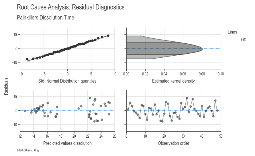Root Cause Analysis - Residuals Residual diagnostics: 4-panel analysis validating model assumptions

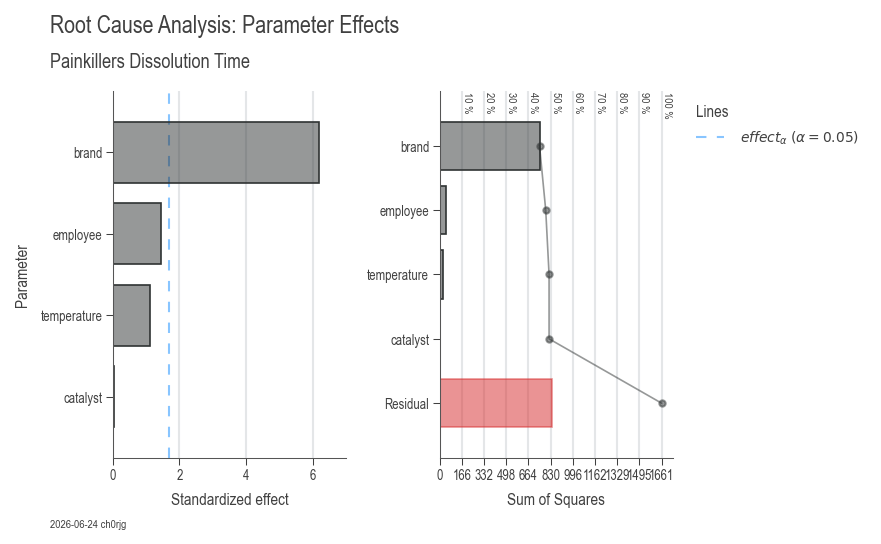Root Cause Analysis - Parameters Parameter effects: ANOVA table, effect sizes, and statistical significance

What You Get¶

ResidualsCharts (Model Validation)¶

Ensures your model assumptions are valid:

Residuals vs Fitted: Check for patterns (should be random scatter)
Q-Q Plot: Verify normality of residuals
Scale-Location: Check homoscedasticity (constant variance)
Residuals vs Leverage: Identify influential outliers

ParameterRelevanceCharts (Factor Analysis)¶

Shows which factors matter:

Parameter estimates with confidence intervals
Effect sizes and statistical significance
ANOVA table (F-statistics and p-values)
R² values (model fit quality)

Automatic interpretation includes: - Significant vs non-significant factors - Effect magnitude and direction - Model quality metrics (R², adjusted R², predicted R²) - Residual analysis diagnostics

Understanding the Output¶

ANOVA Table¶

The ANOVA table shows which factors significantly affect your output:

Source	DF	SS	MS	F	p-value	η²
Factor A	2	1360.7	680.4	10.2	0.001	0.58
Factor B	1	234.5	234.5	3.5	0.082	0.12
Residual	15	1001.8	66.8	-	-	0.42

Interpretation: - p-value < 0.05: Factor is statistically significant (reject H₀) - η² (eta-squared): Proportion of variance explained (effect size) - F-statistic: Ratio of explained to unexplained variance

Goodness-of-Fit Metrics¶

R²: Proportion of variance explained (0-1, higher is better)
Adjusted R²: R² penalized for model complexity
Predicted R²: Cross-validation estimate (avoid overfitting)
Target: R² > 0.7 for good fit, adjusted R² ≈ predicted R²

Real-World Example: Quality Investigation¶

import daspi as dsp

# Load manufacturing data
df = dsp.load_dataset("painkillers-dissolution")

# Investigate dissolution time issues
model = dsp.LinearModel(
    source=df,
    target="dissolution",
    factors=[
        "employee",    # Categorical: who made it
        "stirrer",     # Categorical: equipment type
        "brand",       # Categorical: material supplier
        "catalyst",    # Categorical: process variant
        "water"        # Categorical: water type
    ],
    covariates=[
        "temperature",  # Continuous: process temperature
        "preparation"   # Continuous: prep time
    ],
    order=2,  # Include interaction effects
    alpha=0.05
)

# Backward elimination removes non-significant factors
df_elimination = model.recursive_elimination()
print(df_elimination)

# Visualize final model
residuals = dsp.ResidualsCharts(model
    ).plot(
    ).stripes(
    ).label(
        fig_title="Dissolution Time Root Cause Analysis",
        sub_title="Residual Diagnostics",
        info=True
    )

parameters = dsp.ParameterRelevanceCharts(model
    ).plot(
    ).stripes(
    ).label(
        fig_title="Dissolution Time Root Cause Analysis", 
        sub_title="Parameter Effects",
        info=True
    )

# Get ANOVA table
print(model.anova())

# Get parameter estimates
print(model.params())

Advanced Analysis¶

Interaction Effects¶

Interactions occur when the effect of one factor depends on the level of another:

# Include 2-way interactions
model = dsp.LinearModel(
    source=df,
    target="yield",
    factors=["temperature", "pressure"],
    order=2  # Includes Temperature × Pressure
)

Interpretation: - Significant interaction: Optimize factors together - Non-significant interaction: Optimize factors independently

Categorical vs Continuous Factors¶

model = dsp.LinearModel(
    source=df,
    target="output",
    factors=["machine", "operator"],  # Categorical
    covariates=["speed", "feed"]      # Continuous
)

Difference: - Factors: Discrete levels (compare groups) - Covariates: Continuous (regression relationship)

Model Comparison¶

import pandas as pd

# Fit multiple models
model1 = dsp.LinearModel(source=df, target="y", factors=["A", "B"])
model2 = dsp.LinearModel(source=df, target="y", factors=["A", "B", "C"])
model3 = dsp.LinearModel(source=df, target="y", factors=["A", "B", "C"], order=2)

# Compare quality metrics
comparison = pd.DataFrame({
    'Model': ['A+B', 'A+B+C', 'A+B+C+interactions'],
    'R²': [model1.r2, model2.r2, model3.r2],
    'Adj R²': [model1.r2_adj, model2.r2_adj, model3.r2_adj],
    'Pred R²': [model1.r2_pred, model2.r2_pred, model3.r2_pred]
})
print(comparison)

Interpretation Guidelines¶

Residual Analysis¶

✅ Good model: - Residuals randomly scattered (no patterns) - Q-Q plot follows diagonal line (normal) - No influential outliers (Cook's distance < 1)

❌ Problem indicators: - Curved pattern → missing interaction or non-linear term - Funnel shape → heteroscedasticity (transformation needed) - Points far from Q-Q line → outliers or non-normality

Statistical Significance¶

p-value < 0.05: Factor is significant - Effect is real (not due to chance) - Include in final model

p-value ≥ 0.05: Factor is not significant - Effect indistinguishable from noise - Consider removing (simplify model)

Effect Size (η²)¶

η² > 0.14: Large effect (factor has major impact)
0.06 < η² < 0.14: Medium effect
η² < 0.06: Small effect (may not be practically important)

Common Issues & Solutions¶

Issue: Non-normal residuals¶

Causes: Outliers, wrong model structure, non-normal data
Solutions: 1. Check for outliers and investigate 2. Try transformation (log, sqrt, Box-Cox) 3. Add missing interaction terms

Issue: Low R² despite significant factors¶

Causes: High inherent variation, missing factors
Solutions: 1. Check measurement system capability (Gage R&R) 2. Identify additional factors (process mapping, brainstorming) 3. Improve process control to reduce noise

Issue: Adjusted R² << Predicted R²¶

Cause: Overfitting (model too complex)
Solution: Use backward elimination, reduce model complexity

Issue: Multicollinearity warning¶

Cause: Highly correlated predictors
Solution: Remove redundant factors, use VIF analysis

Step-by-Step Workflow¶

1. Data Preparation¶

# Load and inspect data
df = dsp.load_dataset("your_data")
print(df.info())
print(df.describe())

2. Fit Initial Model¶

# Include all suspected factors
model = dsp.LinearModel(
    source=df,
    target="output",
    factors=["factorA", "factorB", "factorC"],
    covariates=["covariate1"],
    order=1  # Start without interactions
)

3. Check Model Fit¶

# Visualize residuals
dsp.ResidualsCharts(model).plot().stripes().label(info=True)

# Check metrics
print(f"R² = {model.r2:.3f}")
print(f"Adj R² = {model.r2_adj:.3f}")
print(f"Pred R² = {model.r2_pred:.3f}")

4. Simplify Model¶

# Remove non-significant factors
model.recursive_elimination(alpha=0.05)

# Review final model
print(model.anova())

5. Interpret Results¶

# Visualize parameter effects
dsp.ParameterRelevanceCharts(model).plot().stripes().label(info=True)

# Get estimates with confidence intervals
params = model.params()
print(params[['estimate', 'ci_low', 'ci_upp', 'p']])

6. Validate & Implement¶

Verify findings with confirmation runs
Implement process changes based on key factors
Monitor with SPC (Workflow 3)

Next Steps¶

Workflow 1: Capability Analysis — Verify improvements
Workflow 3: SPC Charts — Monitor sustained improvement
Related: DOE Guide — Design experiments to test factor effects
Related: Hypothesis Testing — Statistical testing fundamentals